I completed two major research projects as an undergrad at the College of Wooster.
Senior Independent Study (Orals – Paper)
At the College of Wooster I completed an Independent Study entitled “The SIAM 100.0000000-Digit Challenge: A Study In High Accuracy Numerical Computing Using Interval Analysis and Mathematica.” I considered three of the ten problems.
- A photon moving at speed 1 in the xy-plane starts at time t = 0 at (x, y) = (1/2, 1/10) heading due east. Around every integer lattice point (i, j) in the plane, a circular mirror of radius 1/3 has been erected. How far from (0, 0) is the photon at t = 10?
- Find the global minimum of the function
\[
\begin{split}f(x,y) = e^{\sin(50x)} &+\sin(60e^y) + \sin(70 \sin x) \\ &+\sin\bigl(\sin(80y)\bigr) – \sin(\bigl(10(x+y)\bigr) + \frac{x^2+y^2}{4}.\end{split}
\] - Let A be the 20000 x 20000 matrix whose entries are zero everywhere except for the primes 2, 3, 5, 7,…, 224737 along the main diagonal and the number 1 in all the positions \(a_{ij}\) with |i − j| = 1, 2, 4, 8,…, 16384. What is the (1, 1) entry of \(A^{-1}\)?
So how would we attack these problems? I’ll give a brief summary of why the problem is hard and how it is solved. All of these solutions can be found in the SIAM 100-Digit Challenge Book.
Problem 1
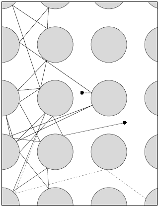
At first we are able to estimate the path the photon will take by using a simple geometric argument with trial-and-error. The problem we run into is whether the path we found is reliable due to decreased precision. For example, in the picture below we see that at time 20, the machine-precision trajectory (solid) is at a very different point than one following the path (dashed) computed with enough precision to guarantee correctness.
To prevent this from happening, we take the algorithm we used to solve the problem using machine precision and transform it into a naive interval algorithm; that is, we place small intervals around our inputs and replace each operation by the corresponding interval operation. The result is an interval enclosure of the photon’s position at time 10. If the interval is not small enough or the required precision is too low, then just restart the algorithm and reduce the interval enclosure by a factor of 10 about the initial condition.
Problem 2
We may take the largest enclosing region amongst all the terms in f(x,y) (except the last one) which leads us to believe the global minimum lies within the square [-1,1] x [-1,1]. Although f(x,y) may look like a quadratic surface globally, the trigonometric elements add extreme complexity as seen in the picture below.
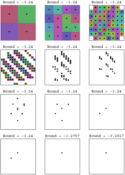
A simple approach is to use a fine grid and approximate the function at every point on this grid. The importance is that this gets us an upper bound on the minimum. Another approach for this problem is to use a genetic algorithm which utilizes this upper bound. The concern with genetic algorithms is their tendency to converge toward local minima rather than the global minimum of the problem. Instead, to get verifiably correct solutions to our problem, we will again use an interval algorithm. We divide our region [-1,1] x [-1,1] into subrectangles and retain only those subrectangles T that have a possibility of containing the global minimum. Let f[T] denote the enclosing interval for \(\bigl\{f(t) : t \in T\bigr\}\). At each iteration, the subrectangles become candidates to only if they pass the three conditions below:
- f[T] is an interval whose left end is less than or equal to the current upper bound on the absolute minimum.
- \(f_x[T]\) is an interval whose left end is negative and right end is positive.
- \(f_y[T]\) is an interval whose left end is negative and right end is positive.
This “search-and-destroy” procedure can be run until the desired precision is met.
Problem 3
In general, inverting a matrix is a bad idea and most algorithms are usually numerically unstable and have a chance of introducing approximation errors. A reformulation of this problem is to solve the linear equation of the form
\[
Ax = \mathbf{b} \text{ with } \mathbf{b} = (1,0,\ldots, 0)^T \text{ and } x = (x_1, \ldots, x_n)^T.
\]
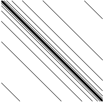
To work with such a large matrix we use Mathematica‘s built in SparseArray function. The reason we use this is because there are 554,466 nonzero entries which account for about 0.14% of the total. The sparsity pattern of A is illustrated below.

To solve this problem efficiently, we can apply the conjugate gradient method and precondition the system. Some nice preconditioners for this system are a matrix of the diagonal entries or an incomplete Cholesky factorization.
Research Experience for Undergraduates (Link – Talk – Paper)
During the summer in 2006 I participated in a REU at the University of Akron where we wrote a paper entitled, “Self-Similar Tilings of Nilpotent Lie Groups.” We described a set of conditions for self-similar tilings (which typically had fractal boundaries) to exist over nilpotent Lie groups. The major result we proved was that given an expansive automorphism that preserves some lattice, we can construct a self-similar tile. Once we have this result for all nilpotent Lie groups, we examine the Heisenberg group, a specific example. In the Heisenberg group, we can describe precisely the form of all automorphisms, and in particular we can describe all automorphisms with the property of being an expansive map. We also classify all lattices in the three-dimensional Heisenberg group, which allows us to construct specific examples of self-similar tilings on this group, which can be represented as plots in \(\mathbb{R}^3\).


