Computational Real Algebraic Geometry
The basic elements of study in real algebraic geometry are semi-algebraic sets; sets defined by polynomial equations and inequalities over \(\mathbb{R}^n\). One fundamental problem is the connectivity problem: determining whether two given points lie in a same connected component of a given semi-algebraic set S. We want to develop an algorithm to solve the following problem.
| Input: | \(f \in \mathbb{Z}[x_1, \dotsc, x_n]\) |
| \(p_1, p_2\), two points in \( \{ f \neq 0\}\) | |
| Output: | True, if and only if \(p_1\) and \(p_2\) are in a same connected component of \( \{ f \neq 0\}\). |
Here, \( \{ f \neq 0\}\) is shorthand notation for the set \(\{ (x_1, \dotsc, x_n) \vert f(x_1, \dotsc, x_n) \neq 0\}\). For example, suppose \(f(x_1, x_2) = x_1^2 + x_2^2 – 1\) where \(S = \{ f \neq 0\}\). We show the set S as the white region below. The black curve is the complement of the set S, the set of points on the unit circle centered at the origin. The points \(p_1\) and \(p_2\) are the blue and green point, respectively. Notice, that the black curve splits \(\mathbb{R}^2\) in to two distinct regions which we call (semi-algebraic) connected components.
Drag the blue and green points around. Notice how the answer changes when the points are in different regions.
The interactive demo above shows we can solve a very simple instance of this problem. However, solving this problem for more interesting sets S is a very active research area. Many important or non-trivial problems in science and engineering can be reduced to the problem of deciding connectivity properties of semi-algebraic sets. The original motivation came from robot motion planning where one tries to decide collision-free motions for a robot in an environment filled with obstacles. The free space in which the robot can move can be modeled as a semi-algebraic set. Then one wants to know whether a robot can move from an initial configuration (a starting point) to a final configuration (an ending point) within the free space in a continuous motion. If this is true, one must find such a continuous trajectory. Motion planning problems show up in other diverse contexts such as computational biology, virtual prototyping in manufacturing, architectural design, aerospace engineering, and computational geography.
My thesis provides correctness results for a method which solves the problem above. The method first creates a “skeleton” of the set \(\{ f \neq 0\} \), called a connectivity path, illustrated in red in the figure below. Here, we are using \(f(x_1, x_2) = x_1^3 -x_1^2 + x_2^2\).
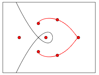
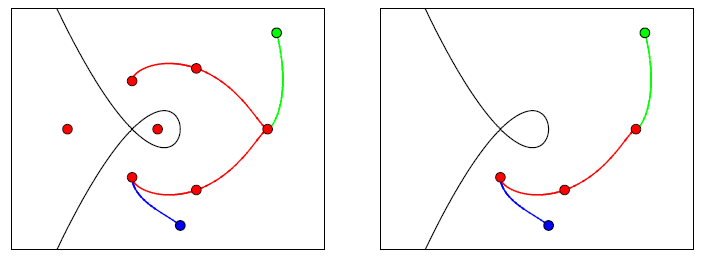
To develop this connectivity path, we create a function g, called a routing function, and connect a particular subset of the critical points of g, called routing points (red points), using trajectories of \(\nabla g\). In my thesis I develop an algorithm to create a routing function in finite time and show the connectivity path is connected in each connected component of \(\{ f \neq 0\} \). Since the connectivity path is connected in each component, a connectivity query can be answered by connecting the input points to the connectivity path using trajectories of \(\nabla g\). The trajectories of \(\nabla g\) for two sample input points (in blue and green) are shown in the left figure below. I illustrate a path connecting the input points (in blue and green) in a connected component using the connectivity path in the right figure below. We expect the length of this path to be finite.
I am interested in several questions related to this algorithm.
- What is a “good” upper bound on the length of the shortest path connecting the input points in a connected component using the connectivity path? A pessimistic upper bound on the length of this path is given in the thesis.
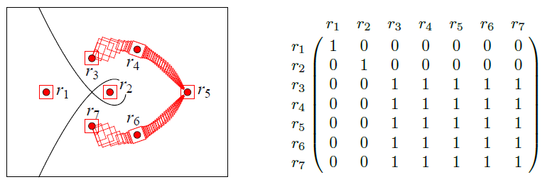
- How do we trace these trajectories rigorously? Imagining the connectivity path as a graph G, whose vertices are the routing points and whose edges are the trajectories of \(\nabla g\), the connectivity matrix of g is the reflexive, symmetric, transitive closure of the adjacency matrix of G. We desire to solve the following problem.
Input: g, a routing function. Output: M, connectivity matrix of g. A possible approach to this problem is to design an algorithm that utilizes interval arithmetic to create a path of interconnected boxes bounding the connectivity path. Labeling the routing points of g as \(r_1, \dotsc, r_7\), we illustrate such a path in the figure below along with the corresponding connectivity matrix.
A necessary first step would be to implement a rigorous ODE solver in C++ using the Boost library and then run computational tests.
- I am also interested in questions about classification of routing functions and studying properties of routing points.
Symbolic Computation
Over several summers, I mentored three graduate students, each covering different problems in the field of symbolic computation. The first student studied root separation bounds.
| Input: | \(f = a_d \prod_{i=1}^d (x- \alpha_i)\). |
| Output: | \(B \geq 0\) such that for all \(i \neq j\), \(\lvert\alpha_i – \alpha_j\rvert \geq B\). |
A future goal is to obtain a bound B which behaves well under root translation, root scaling, and polynomial scaling. A second goal is to create tighter bounds. Some bounds are too small to be practical, so their use is generally restricted to complexity analysis.
The second problem, related to cyclotomic polynomials. Let g(f) denote the maximum of the differences (gaps) between two consecutive exponents in a polynomial f. The problem is to come up with “nice” expressions for \(g(\Phi_n)\) and \(g(\Psi_n)\) where \(\Phi_n\) and \(\Psi_n\) denote the n-th cyclotomic polynomial and n-th inverse cyclotomic polynomial, respectively. Previous work has been done on the case when n is a product of odd primes. Certainly much more research can be done for other choices of n.
The third problem related to computing derivatives of an implicitly defined function. The problem is, given \(f(x, y) = 0\), give a closed form expression for \(\frac{d^ny}{dx^n}\) in terms of the derivatives of f. Despite being a longstanding problem, a solution was first presented in 2012. A future goal is to come up with a simpler closed form expression than the one presented in that paper.
Optimization
During my Master’s degree, I studied the nonlinear resource allocation problem.
$$
\begin{array}{rll}
\min &{\displaystyle f(x) := \sum f_i(x_{i})} &\\[1.25em]
\textrm{subject to} &{\displaystyle g(x) := \sum g_i(x_i) \leq b}, & \\[1.25em]
& \ell_i \leq x_i \leq u_i, &i = 1, \dotsc, n,
\end{array}
$$
where x, \(\ell\), and u are n-vectors of real numbers, b is a real scalar, and the functions \(f_i\) and \(g_i\) are
convex and twice differentiable on an open set containing the interval \([\ell_i, u_i]\). This problem has a long history and diverse applications. Moreover, this problem often serves as a subproblem that is integrated into a much larger model and solved numerous times. Hence, the development of efficient algorithms for this problem is extremely important. A fast method for solving this problem was presented by myself and a coauthor. There are several avenues for future research.
- We can study the specialized problem when the variables are integral, and compare the various branch-and-bound methods which can be applied to this problem.
- We can identify other optimization problems whose optimality conditions can be simplified algebraically in a way similar to the nonlinear resource allocation problem. These simplifications will then be integrated into an interior point method.
Technology in the Classroom
Currently, I assign Mathematica labs that must be graded by hand. I believe a future improvement would be the inclusion of automated grading with immediate feedback. At North Carolina State University they have a program called eMarker, originally called eGrader. This is a neat bit of software that randomly generates Maple assignments based on a template, then automatically grades the submitted worksheet and, most importantly, gives immediate feedback on any errors. The eMarker software seems to be well received by the students at NC State. I believe a similar bit of software that uses Mathematica as the back end would be much more powerful and would allow for better types of assessment than the Maple version.
I am currently investigating what makes a “good” instructional video. For example, I will be studying whether students prefer a video that include the instructors face or not, or whether they prefer pauses in a presentation.